# graphlayouts
**Repository Path**: chens1209/graphlayouts
## Basic Information
- **Project Name**: graphlayouts
- **Description**: new layout algorithms for network visualizations in R
- **Primary Language**: Unknown
- **License**: Not specified
- **Default Branch**: master
- **Homepage**: None
- **GVP Project**: No
## Statistics
- **Stars**: 0
- **Forks**: 0
- **Created**: 2020-08-11
- **Last Updated**: 2020-12-20
## Categories & Tags
**Categories**: Uncategorized
**Tags**: None
## README
# graphlayouts  [](https://travis-ci.org/schochastics/graphlayouts)
[](https://ci.appveyor.com/project/schochastics/smglr)
[](https://cran.r-project.org/package=graphlayouts)
[](https://www.tidyverse.org/lifecycle/#stable)
[](https://CRAN.R-project.org/package=graphlayouts)
This package implements some graph layout algorithms that are not
available in `igraph`.
**A detailed introductory tutorial for graphlayouts and ggraph can be
found [here](http://mr.schochastics.net/netVizR.html).**
The package implements the following algorithms:
- Stress majorization
([Paper](https://graphviz.gitlab.io/_pages/Documentation/GKN04.pdf))
- Quadrilateral backbone layout
([Paper](http://jgaa.info/accepted/2015/NocajOrtmannBrandes2015.19.2.pdf))
- flexible radial layouts
([Paper](http://jgaa.info/accepted/2011/BrandesPich2011.15.1.pdf))
- sparse stress ([Paper](https://arxiv.org/abs/1608.08909))
- pivot MDS
([Paper](https://kops.uni-konstanz.de/bitstream/handle/123456789/5741/bp_empmdsld_06.pdf?sequence=1&isAllowed=y))
- dynamic layout for longitudinal data
([Paper](https://kops.uni-konstanz.de/bitstream/handle/123456789/20924/Brandes_209246.pdf?sequence=2))
- spectral layouts (adjacency/Laplacian)
## Install
``` r
# dev version
remotes::install_github("schochastics/graphlayouts")
#CRAN
install.packages("graphlayouts")
```
## Stress Majorization: Connected Network
*This example is a bit of a special case since it exploits some weird
issues in igraph.*
``` r
library(igraph)
library(ggraph)
library(graphlayouts)
set.seed(666)
pa <- sample_pa(1000,1,1,directed = F)
ggraph(pa,layout = "nicely")+
geom_edge_link0(width=0.2,colour="grey")+
geom_node_point(col="black",size=0.3)+
theme_graph()
```
[](https://travis-ci.org/schochastics/graphlayouts)
[](https://ci.appveyor.com/project/schochastics/smglr)
[](https://cran.r-project.org/package=graphlayouts)
[](https://www.tidyverse.org/lifecycle/#stable)
[](https://CRAN.R-project.org/package=graphlayouts)
This package implements some graph layout algorithms that are not
available in `igraph`.
**A detailed introductory tutorial for graphlayouts and ggraph can be
found [here](http://mr.schochastics.net/netVizR.html).**
The package implements the following algorithms:
- Stress majorization
([Paper](https://graphviz.gitlab.io/_pages/Documentation/GKN04.pdf))
- Quadrilateral backbone layout
([Paper](http://jgaa.info/accepted/2015/NocajOrtmannBrandes2015.19.2.pdf))
- flexible radial layouts
([Paper](http://jgaa.info/accepted/2011/BrandesPich2011.15.1.pdf))
- sparse stress ([Paper](https://arxiv.org/abs/1608.08909))
- pivot MDS
([Paper](https://kops.uni-konstanz.de/bitstream/handle/123456789/5741/bp_empmdsld_06.pdf?sequence=1&isAllowed=y))
- dynamic layout for longitudinal data
([Paper](https://kops.uni-konstanz.de/bitstream/handle/123456789/20924/Brandes_209246.pdf?sequence=2))
- spectral layouts (adjacency/Laplacian)
## Install
``` r
# dev version
remotes::install_github("schochastics/graphlayouts")
#CRAN
install.packages("graphlayouts")
```
## Stress Majorization: Connected Network
*This example is a bit of a special case since it exploits some weird
issues in igraph.*
``` r
library(igraph)
library(ggraph)
library(graphlayouts)
set.seed(666)
pa <- sample_pa(1000,1,1,directed = F)
ggraph(pa,layout = "nicely")+
geom_edge_link0(width=0.2,colour="grey")+
geom_node_point(col="black",size=0.3)+
theme_graph()
```
 ``` r
ggraph(pa,layout="stress")+
geom_edge_link0(width=0.2,colour="grey")+
geom_node_point(col="black",size=0.3)+
theme_graph()
```
``` r
ggraph(pa,layout="stress")+
geom_edge_link0(width=0.2,colour="grey")+
geom_node_point(col="black",size=0.3)+
theme_graph()
```
 ## Stress Majorization: Unconnected Network
Stress majorization also works for networks with several components. It
relies on a bin packing algorithm to efficiently put the components in a
rectangle, rather than a circle.
``` r
set.seed(666)
g <- disjoint_union(
sample_pa(10,directed = F),
sample_pa(20,directed = F),
sample_pa(30,directed = F),
sample_pa(40,directed = F),
sample_pa(50,directed = F),
sample_pa(60,directed = F),
sample_pa(80,directed = F)
)
ggraph(g,layout = "nicely") +
geom_edge_link0() +
geom_node_point() +
theme_graph()
```
## Stress Majorization: Unconnected Network
Stress majorization also works for networks with several components. It
relies on a bin packing algorithm to efficiently put the components in a
rectangle, rather than a circle.
``` r
set.seed(666)
g <- disjoint_union(
sample_pa(10,directed = F),
sample_pa(20,directed = F),
sample_pa(30,directed = F),
sample_pa(40,directed = F),
sample_pa(50,directed = F),
sample_pa(60,directed = F),
sample_pa(80,directed = F)
)
ggraph(g,layout = "nicely") +
geom_edge_link0() +
geom_node_point() +
theme_graph()
```
 ``` r
ggraph(g, layout = "stress",bbox = 40) +
geom_edge_link0() +
geom_node_point() +
theme_graph()
```
``` r
ggraph(g, layout = "stress",bbox = 40) +
geom_edge_link0() +
geom_node_point() +
theme_graph()
```
 ## Backbone Layout
Backbone layouts are helpful for drawing hairballs.
``` r
set.seed(665)
#create network with a group structure
g <- sample_islands(9,40,0.4,15)
g <- simplify(g)
V(g)$grp <- as.character(rep(1:9,each=40))
ggraph(g,layout = "stress")+
geom_edge_link0(colour=rgb(0,0,0,0.5),width=0.1)+
geom_node_point(aes(col=grp))+
scale_color_brewer(palette = "Set1")+
theme_graph()+
theme(legend.position = "none")
```
## Backbone Layout
Backbone layouts are helpful for drawing hairballs.
``` r
set.seed(665)
#create network with a group structure
g <- sample_islands(9,40,0.4,15)
g <- simplify(g)
V(g)$grp <- as.character(rep(1:9,each=40))
ggraph(g,layout = "stress")+
geom_edge_link0(colour=rgb(0,0,0,0.5),width=0.1)+
geom_node_point(aes(col=grp))+
scale_color_brewer(palette = "Set1")+
theme_graph()+
theme(legend.position = "none")
```
 The backbone layout helps to uncover potential group structures based on
edge embeddedness and puts more emphasis on this structure in the
layout.
``` r
bb <- layout_as_backbone(g,keep=0.4)
E(g)$col <- F
E(g)$col[bb$backbone] <- T
ggraph(g,layout="manual",x=bb$xy[,1],y=bb$xy[,2])+
geom_edge_link0(aes(col=col),width=0.1)+
geom_node_point(aes(col=grp))+
scale_color_brewer(palette = "Set1")+
scale_edge_color_manual(values=c(rgb(0,0,0,0.3),rgb(0,0,0,1)))+
theme_graph()+
theme(legend.position = "none")
```
The backbone layout helps to uncover potential group structures based on
edge embeddedness and puts more emphasis on this structure in the
layout.
``` r
bb <- layout_as_backbone(g,keep=0.4)
E(g)$col <- F
E(g)$col[bb$backbone] <- T
ggraph(g,layout="manual",x=bb$xy[,1],y=bb$xy[,2])+
geom_edge_link0(aes(col=col),width=0.1)+
geom_node_point(aes(col=grp))+
scale_color_brewer(palette = "Set1")+
scale_edge_color_manual(values=c(rgb(0,0,0,0.3),rgb(0,0,0,1)))+
theme_graph()+
theme(legend.position = "none")
```
 ## Radial Layout with Focal Node
The function `layout_with_focus()` creates a radial layout around a
focal node. All nodes with the same distance from the focal node are on
the same circle.
``` r
library(igraphdata)
library(patchwork)
data("karate")
p1 <- ggraph(karate,layout = "focus",focus = 1) +
draw_circle(use = "focus",max.circle = 3)+
geom_edge_link0(edge_color="black",edge_width=0.3)+
geom_node_point(aes(fill=as.factor(Faction)),size=2,shape=21)+
scale_fill_manual(values=c("#8B2323", "#EEAD0E"))+
theme_graph()+
theme(legend.position = "none")+
coord_fixed()+
labs(title= "Focus on Mr. Hi")
p2 <- ggraph(karate,layout = "focus",focus = 34) +
draw_circle(use = "focus",max.circle = 4)+
geom_edge_link0(edge_color="black",edge_width=0.3)+
geom_node_point(aes(fill=as.factor(Faction)),size=2,shape=21)+
scale_fill_manual(values=c("#8B2323", "#EEAD0E"))+
theme_graph()+
theme(legend.position = "none")+
coord_fixed()+
labs(title= "Focus on John A.")
p1+p2
```
## Radial Layout with Focal Node
The function `layout_with_focus()` creates a radial layout around a
focal node. All nodes with the same distance from the focal node are on
the same circle.
``` r
library(igraphdata)
library(patchwork)
data("karate")
p1 <- ggraph(karate,layout = "focus",focus = 1) +
draw_circle(use = "focus",max.circle = 3)+
geom_edge_link0(edge_color="black",edge_width=0.3)+
geom_node_point(aes(fill=as.factor(Faction)),size=2,shape=21)+
scale_fill_manual(values=c("#8B2323", "#EEAD0E"))+
theme_graph()+
theme(legend.position = "none")+
coord_fixed()+
labs(title= "Focus on Mr. Hi")
p2 <- ggraph(karate,layout = "focus",focus = 34) +
draw_circle(use = "focus",max.circle = 4)+
geom_edge_link0(edge_color="black",edge_width=0.3)+
geom_node_point(aes(fill=as.factor(Faction)),size=2,shape=21)+
scale_fill_manual(values=c("#8B2323", "#EEAD0E"))+
theme_graph()+
theme(legend.position = "none")+
coord_fixed()+
labs(title= "Focus on John A.")
p1+p2
```
 ## Radial Centrality Layout
The function `layout_with_centrality` creates a radial layout around the
node with the highest centrality value. The further outside a node is,
the more peripheral it is.
``` r
library(igraphdata)
library(patchwork)
data("karate")
bc <- betweenness(karate)
p1 <- ggraph(karate,layout = "centrality", centrality = bc, tseq = seq(0,1,0.15)) +
draw_circle(use = "cent") +
annotate_circle(bc,format="",pos="bottom") +
geom_edge_link0(edge_color="black",edge_width=0.3)+
geom_node_point(aes(fill=as.factor(Faction)),size=2,shape=21)+
scale_fill_manual(values=c("#8B2323", "#EEAD0E"))+
theme_graph()+
theme(legend.position = "none")+
coord_fixed()+
labs(title="betweenness centrality")
cc <- closeness(karate)
p2 <- ggraph(karate,layout = "centrality", centrality = cc, tseq = seq(0,1,0.2)) +
draw_circle(use = "cent") +
annotate_circle(cc,format="scientific",pos="bottom") +
geom_edge_link0(edge_color="black",edge_width=0.3)+
geom_node_point(aes(fill=as.factor(Faction)),size=2,shape=21)+
scale_fill_manual(values=c("#8B2323", "#EEAD0E"))+
theme_graph()+
theme(legend.position = "none")+
coord_fixed()+
labs(title="closeness centrality")
p1+p2
```
## Radial Centrality Layout
The function `layout_with_centrality` creates a radial layout around the
node with the highest centrality value. The further outside a node is,
the more peripheral it is.
``` r
library(igraphdata)
library(patchwork)
data("karate")
bc <- betweenness(karate)
p1 <- ggraph(karate,layout = "centrality", centrality = bc, tseq = seq(0,1,0.15)) +
draw_circle(use = "cent") +
annotate_circle(bc,format="",pos="bottom") +
geom_edge_link0(edge_color="black",edge_width=0.3)+
geom_node_point(aes(fill=as.factor(Faction)),size=2,shape=21)+
scale_fill_manual(values=c("#8B2323", "#EEAD0E"))+
theme_graph()+
theme(legend.position = "none")+
coord_fixed()+
labs(title="betweenness centrality")
cc <- closeness(karate)
p2 <- ggraph(karate,layout = "centrality", centrality = cc, tseq = seq(0,1,0.2)) +
draw_circle(use = "cent") +
annotate_circle(cc,format="scientific",pos="bottom") +
geom_edge_link0(edge_color="black",edge_width=0.3)+
geom_node_point(aes(fill=as.factor(Faction)),size=2,shape=21)+
scale_fill_manual(values=c("#8B2323", "#EEAD0E"))+
theme_graph()+
theme(legend.position = "none")+
coord_fixed()+
labs(title="closeness centrality")
p1+p2
```
 ## Large graphs
`graphlayouts` implements two algorithms for visualizing large networks
(\<100k nodes). `layout_with_pmds()` is similar to `layout_with_mds()`
but performs the multidimensional scaling only with a small number of
pivot nodes. Usually, 50-100 are enough to obtain similar results to the
full MDS.
`layout_with_sparse_stress()` performs stress majorization only with a
small number of pivots (\~50-100). The runtime performance is inferior
to pivotMDS but the quality is far superior.
A comparison of runtimes and layout quality can be found in the
[wiki](https://github.com/schochastics/graphlayouts/wiki/)
**tl;dr**: both layout algorithms appear to be faster than the fastest
igraph algorithm `layout_with_drl()`.
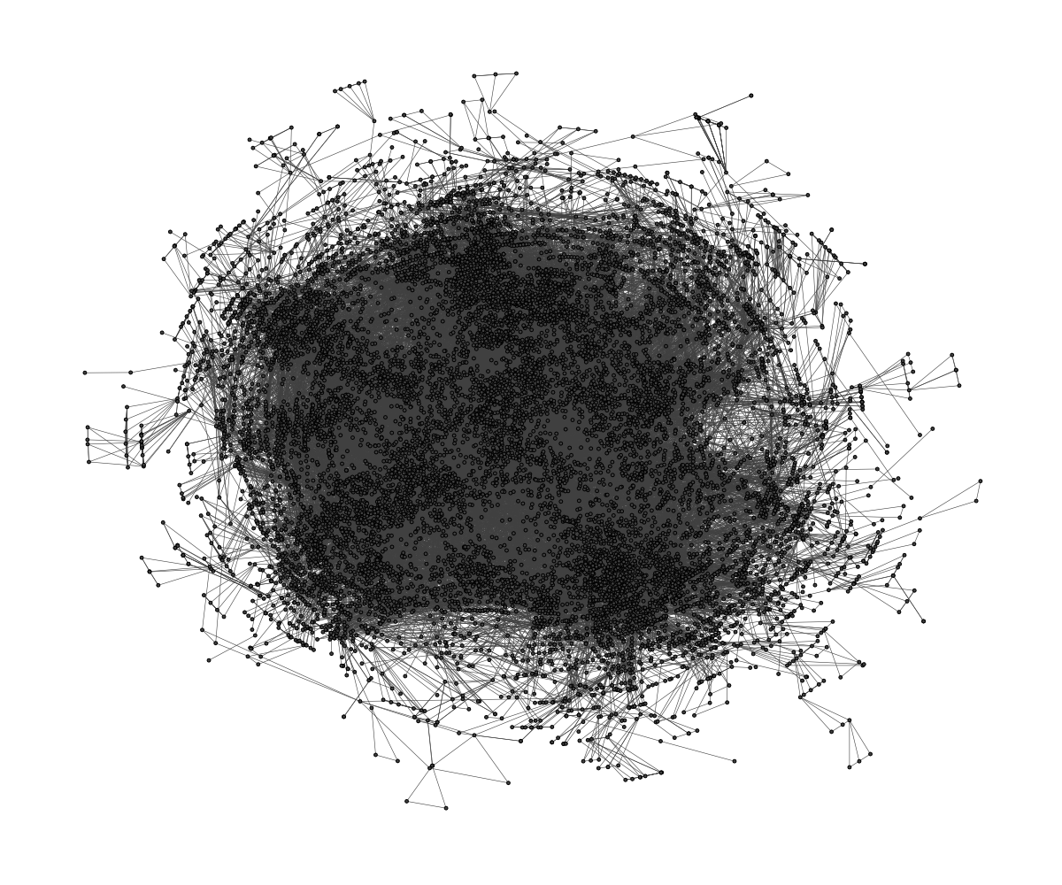
Below are two examples of layouts generated for large graphs using
`layout_with_sparse_stress()`
## Large graphs
`graphlayouts` implements two algorithms for visualizing large networks
(\<100k nodes). `layout_with_pmds()` is similar to `layout_with_mds()`
but performs the multidimensional scaling only with a small number of
pivot nodes. Usually, 50-100 are enough to obtain similar results to the
full MDS.
`layout_with_sparse_stress()` performs stress majorization only with a
small number of pivots (\~50-100). The runtime performance is inferior
to pivotMDS but the quality is far superior.
A comparison of runtimes and layout quality can be found in the
[wiki](https://github.com/schochastics/graphlayouts/wiki/)
**tl;dr**: both layout algorithms appear to be faster than the fastest
igraph algorithm `layout_with_drl()`.
Below are two examples of layouts generated for large graphs using
`layout_with_sparse_stress()`
 A retweet network with 18k nodes and 61k edges
 A co-citation network with 12k nodes and 68k edges
## dynamic layouts
`layout_as_dynamic()` allows you to visualize snapshots of longitudinal
network data. Nodes are anchored with a reference layout and only moved
slightly in each wave depending on deleted/added edges. In this way, it
is easy to track down specific nodes throughout time. Use `patchwork` to
put the individual plots next to each other.
``` r
library(patchwork)
#gList is a list of longitudinal networks.
xy <- layout_as_dynamic(gList,alpha = 0.2)
pList <- vector("list",length(gList))
for(i in 1:length(gList)){
pList[[i]] <- ggraph(gList[[i]],layout="manual",x=xy[[i]][,1],y=xy[[i]][,2])+
geom_edge_link0(edge_width=0.6,edge_colour="grey66")+
geom_node_point(shape=21,aes(fill=smoking),size=3)+
geom_node_text(aes(label=1:50),repel = T)+
scale_fill_manual(values=c("forestgreen","grey25","firebrick"),guide=ifelse(i!=2,FALSE,"legend"))+
theme_graph()+
theme(legend.position="bottom")+
labs(title=paste0("Wave ",i))
}
Reduce("+",pList)+
plot_annotation(title="Friendship network",theme = theme(title = element_text(family="Arial Narrow",face = "bold",size=16)))
```
A co-citation network with 12k nodes and 68k edges
## dynamic layouts
`layout_as_dynamic()` allows you to visualize snapshots of longitudinal
network data. Nodes are anchored with a reference layout and only moved
slightly in each wave depending on deleted/added edges. In this way, it
is easy to track down specific nodes throughout time. Use `patchwork` to
put the individual plots next to each other.
``` r
library(patchwork)
#gList is a list of longitudinal networks.
xy <- layout_as_dynamic(gList,alpha = 0.2)
pList <- vector("list",length(gList))
for(i in 1:length(gList)){
pList[[i]] <- ggraph(gList[[i]],layout="manual",x=xy[[i]][,1],y=xy[[i]][,2])+
geom_edge_link0(edge_width=0.6,edge_colour="grey66")+
geom_node_point(shape=21,aes(fill=smoking),size=3)+
geom_node_text(aes(label=1:50),repel = T)+
scale_fill_manual(values=c("forestgreen","grey25","firebrick"),guide=ifelse(i!=2,FALSE,"legend"))+
theme_graph()+
theme(legend.position="bottom")+
labs(title=paste0("Wave ",i))
}
Reduce("+",pList)+
plot_annotation(title="Friendship network",theme = theme(title = element_text(family="Arial Narrow",face = "bold",size=16)))
```
 ## Layout manipulation
The functions `layout_mirror()` and `layout_rotate()` can be used to
manipulate an existing layout
## Layout manipulation
The functions `layout_mirror()` and `layout_rotate()` can be used to
manipulate an existing layout
